One billion random points. One browser tab. Fans never kicked in.

I built a Monte Carlo π approximation — scatter random points in a unit square, count how many land inside a quarter circle, multiply the ratio by four, and you get π. Simple math. I wanted to see how far a browser could push it, so I typed in a billion and hit start. The page stayed responsive the entire time.

This post is not about Monte Carlo. It is about the rendering architecture that made that number possible.

The Naive Approach Dies Fast

The obvious way to draw points on a canvas is the Canvas 2D API. For each point, you call fillRect() or arc(), set a fill color, and move on. This works fine for a few thousand points.

At scale, it falls apart. Each Canvas API call has overhead: style parsing, state machine transitions, rasterization per shape. At one million points you feel the lag. At one billion, the tab would simply crash — you cannot store one billion point objects in memory and you cannot make one billion draw calls on the main thread.

The project needed two separate rendering pipelines: one optimized for visual feedback, one optimized for raw throughput. The choice depends on whether you want to watch the simulation happen or just want the result.

Pipeline 1: Realtime Compositing

The realtime mode is designed for watching. Points appear in batches — 10 per frame at normal speed, 100 at fast — so you see the quarter circle fill up gradually. This is where the compositing pattern matters.

The problem with drawing incrementally on a single canvas is that you need to redraw the static elements (grid lines, axis labels, the quarter circle arc) every frame. If you draw dots directly onto the main canvas and then redraw the grid, the grid covers the dots. If you draw the grid first and then all the dots, you are redrawing every dot every frame.

The solution is an offscreen buffer:

// Initialize an invisible canvas as the dot buffer
const buffer = document.createElement('canvas');
buffer.width = CANVAS_SIZE;
buffer.height = CANVAS_SIZE;
const bufCtx = buffer.getContext('2d');

New dots are drawn only onto this buffer. The buffer accumulates — it never gets cleared between frames. Each animation frame, the visible canvas is redrawn from scratch: static elements first, then the entire buffer composited on top in a single drawImage call:

// Only draw NEW dots onto the buffer (incremental)
for (let i = startIdx; i < points.length; i++) {
  const { x, y, inside } = points[i];
  const px = PADDING + x * PLOT_SIZE;
  const py = PADDING + (1 - y) * PLOT_SIZE;

  bufCtx.fillStyle = inside
    ? 'rgba(2, 132, 199, 0.85)' // blue — inside the circle
    : 'rgba(219, 39, 119, 0.7)'; // pink — outside
  bufCtx.fillRect(px - 1, py - 1, 2, 2);
}

// Composite: static layer + dot buffer
drawStaticElements(ctx);
ctx.drawImage(buffer, 0, 0);

The key detail is startIdx. The component tracks how many dots have already been drawn to the buffer. Each frame, it only draws the new batch. Ten or a hundred fillRect calls per frame, regardless of how many dots are already on screen. The buffer holds the history.

This keeps frame times constant. Whether you have 100 dots or 100,000 on screen, each frame does the same amount of work: draw the new batch to the buffer, clear the main canvas, paint the static layer, composite the buffer. Smooth at any point count.

Pipeline 2: Worker Pixel Buffer

The realtime pipeline is great for watching, but it tops out at around a million points before the point array itself becomes a memory problem. For the serious numbers — one billion — you do not need animation. You need raw compute.

The non-realtime mode moves everything to a Web Worker. No Canvas API at all. The worker operates directly on a Uint8ClampedArray — a flat array of RGBA pixel values:

const pixels = new Uint8ClampedArray(CANVAS_SIZE * CANVAS_SIZE * 4);
let insideCount = 0;

for (let i = 0; i < sampleSize; i++) {
  const x = Math.random();
  const y = Math.random();
  const inside = x * x + y * y <= 1;
  if (inside) insideCount++;

  // Map to canvas coordinates and write pixels directly
  const px = (PADDING + x * PLOT_SIZE) | 0;
  const py = (PADDING + (1 - y) * PLOT_SIZE) | 0;

  for (let dy = 0; dy < 2; dy++) {
    for (let dx = 0; dx < 2; dx++) {
      const idx = ((py + dy) * CANVAS_SIZE + (px + dx)) * 4;
      pixels[idx] = inside ? 2 : 219; // R
      pixels[idx + 1] = inside ? 132 : 39; // G
      pixels[idx + 2] = inside ? 199 : 119; // B
      pixels[idx + 3] = 210; // A
    }
  }
}

There are a few things happening here that make the billion-point run possible.

No point storage. The realtime mode pushes every point into an array. At one billion points, that array alone would consume tens of gigabytes. The worker stores nothing. It generates a point, tests it, writes four pixels, and moves on. The only persistent state is the pixel buffer (1 MB for a 500×500 canvas) and a counter.

No Canvas API overhead. Writing pixels[idx] = 199 is a direct memory write. No style parsing, no state machine, no rasterization pipeline. (The | 0 bitwise OR on the coordinates is a micro-optimisation — faster integer truncation than Math.floor().)

No main thread involvement. The Worker runs on its own thread. The main thread stays completely free — the UI is responsive, scroll works, buttons work. The only communication during the run is a progress callback that fires every 1%:

const progressInterval = Math.max(1, Math.floor(sampleSize / 100));

for (let i = 0; i < sampleSize; i++) {
  // ... point generation and pixel writes ...

  if (i % progressInterval === 0) {
    self.postMessage({ type: 'progress', progress: i / sampleSize });
  }
}

At one billion samples, each 1% tick represents ten million iterations. The main thread receives these messages, updates a progress bar, and goes back to idle. That is the entire worker-to-UI contract until the final result lands.

Transferable objects. When the worker finishes, it sends the pixel buffer back to the main thread:

self.postMessage(
  { type: 'done', pixels, insideCount, totalCount: sampleSize },
  [pixels.buffer] // transfer, not copy
);

The second argument — [pixels.buffer] — transfers ownership of the underlying ArrayBuffer to the main thread instead of copying it. For a 1 MB buffer this barely matters, but it is the right pattern. The transfer is O(1) regardless of buffer size.

On the main thread, the buffer becomes an ImageData and gets painted in a single operation:

const imageData = new ImageData(
  new Uint8ClampedArray(pixelBuffer),
  CANVAS_SIZE,
  CANVAS_SIZE
);
tmpCtx.putImageData(imageData, 0, 0);
ctx.drawImage(tmp, 0, 0);

One billion iterations. One putImageData. One drawImage. Done.

Why the Fans Stay Off

I genuinely expected my machine to struggle. One billion iterations of random number generation, multiplication, comparison, and pixel writes — I was ready for the fans to spin up, for the progress bar to crawl, for something to complain. Nothing did. The tab sat there, quietly computing, as if a billion was no different from a thousand.

The reason is architectural. A Web Worker runs on a single thread. It will saturate one CPU core, but modern machines have many cores. The OS does not panic over one busy core. There is no memory pressure because nothing accumulates — the working set is a 1 MB pixel buffer and a few scalar variables. There is no garbage collection pressure because the hot loop allocates nothing. And the main thread is idle, so the browser's own processes (compositor, input handling, rendering) have plenty of room.

Now imagine the naive version: one billion point objects in memory, constant GC pauses, draw calls blocking the main thread. That would absolutely spin up your fans — right before the tab crashes. The difference is not a clever trick. It is the pipeline architecture doing exactly what it was designed to do.

The Visual Output

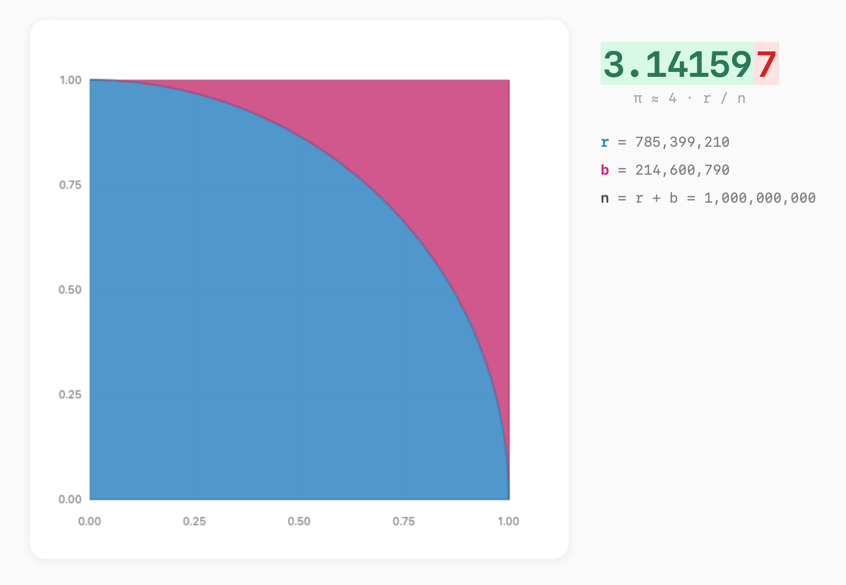
At one billion samples, the quarter circle is solid. You cannot see individual dots anymore — every pixel in the plot area has been written to hundreds of times. The visualization becomes a clean geometric shape: a sharp blue quarter circle against a pink square, with the arc boundary razor-sharp.

785,399,210 points inside the circle. 214,600,790 outside. 3.141597 — five correct decimal places.

Monte Carlo error decreases proportionally to 1/√n. At a billion samples, √n is about 31,623, which puts the expected error around 0.00003 — right at the fifth decimal. To get a sixth, you would need a hundred billion. The method converges, but it converges slowly. That is not a flaw; it is the nature of statistical estimation.

What matters here is that the output at a billion samples is structurally identical to the output at a thousand. The same pixel buffer, the same putImageData call, the same drawImage composite. The pipeline never changed — the scale did. Every architectural decision in this post exists so that the rendering cost stays constant while the sample count goes to whatever number you are brave enough to type in.

What This Comes Down To

Two rendering pipelines for two different goals:

	Realtime	Non-realtime
Where	Main thread	Web Worker
Drawing	Canvas 2D API	Raw pixel array
Memory	O(n) point array	O(1) pixel buffer
Feedback	Animated dots	Progress bar
Scales to	~1M	1B+

The realtime pipeline gives you the experience. The non-realtime pipeline gives you the answer. The compositing pattern (offscreen buffer → single drawImage) keeps the first one smooth. The pixel buffer pattern (direct memory writes → single putImageData) keeps the second one possible. The architecture of each follows directly from what it optimises for.

Try it yourself. Start with realtime mode at 10,000 samples. Watch the dots fill in, watch π converge. Then switch to non-realtime, type in a billion, and see how your machine handles it.